A Spanning Tree, or ST for short, is a subset of a graph that contains every node but not every edge. In this way, the Spanning Tree “spans” the entire graph using only some of the edges.
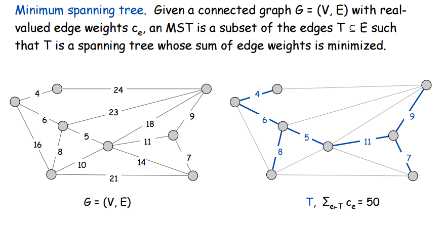
What, then, is a Minumum Spanning Tree? It’s a Spanning Tree that uses the minimum number of existing edges to still be a spanning tree. But we only care about edge-weighted graphs since they’re way better at modelling real life and are therefore an extemely practical data structure. In the case of edge-weighted graphs, a Minimum Spanning Tree (MST) does not use the minimum number of edges but rather minimizes the sum of edge weights. Here’s a picture to illustrate:

There’s something really important to realize about minimum spanning trees: we don’t care how large the sum of the weights are for a given path to and from any node in our MST. We only care about the sum of the weights of all the edges in the MST. No matter how ridiculously huge a particular path in the MST is, if the sum of all the edge-weights in the MST is minimum possible to still reach every node, then it’s the MST.
A cut of a graph is just a subset of nodes. A cycle of a graph is a subset of edges that form a closed loop. The cutset of a cut is the set of edges with only one endpoint in the cut. Some pictures to explain these terms:


Here’s an interesting and (as you’ll soon find) very useful fact: all cutsets and cycles pairs always share an even number of edges (or none at all, but who cares about the trivial case). Not that this counts as proof, but here’s an example of that being true. In the following picture, you will not be able to construct any cycles or cutsets for which this property does not hold.

But why is this true? How can we understand this? Let’s look at a picture which, though it’s not a formal proof, demonstrates why this property is always true for all graphs:

S is the cut, V-S is all nodes not in the cut, C is cutset, and
the cycle is the closed loop of edges with arrows
This picture shows us that each time a cycle enters and exits a cut, it must share two edges with the cutset. Thus a cutset and a cycle must always share 0 or an even number of edges.
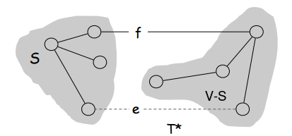
Here’s another interesting fact: In any given graph, for any cut we take of that graph, the minimum edge in that cut’s cutset must be in the MST of the graph as a whole. Why is this necessarily true? We can prove it using one of the greedy analysis strategies discussed at the bottom of the page about interval scheduling, the “exchange strategy”. Basically the proof is as follows and uses the picture below as visualization:

S is a cut, V-S is all nodes not in the cut, T* is the MST shown broken into
two parts awaiting connection by either edge f or e. e is the minimum edge in
S’s cutset, and f is another, non-minimum edge in S’s cutset
T*, the MST, should have only one edge connecting S to V-S. If it had two edges connecting S to V-S, such as f and e, then clearly there would be a cycle and one edge would be removable so we wouldn’t have an MST. The one edge that connects S to V-S that should be in the MST, a.k.a. the one edge is S’s cutset that should be in the MST, is obviously the minimum edge in S’s cutset. If we used any other edge in S’s cutset, T* wouldn’t be the MST.
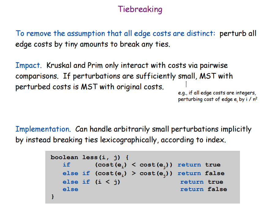
Before I continue to the last property we’re going to talk about, consider that we have assumed that f and e do not have equal weights. It may be that future algorithms we discuss for finding the MST increase in complexity when we cannot make this assumption.
Here’s the final interesting fact/property about graphs: In any given graph, we can be sure that the max-valued edge in any cycle is not in the graph’s MST. This property, just like the property about the minimum edge in any cutset needing to be in a graph’s MST, doesn’t really need any formal proof. Like last time, here’s a visual aid so you can follow the proof visually:
S and V-S are the same as before. Notice that the MST T* has had edge f removed, breaking
it in two “MST-halves” in gray background. Despite this, T* still contains all nodes in the
graph, although cuts S and V-S are unconnected in T* until some connecting edge is added to T*
Say we have some graph with MST T*. And let’s say that edge f is in T* but is also the maximum edge in some cycle L in the graph. If we remove f from T*, T* will now not be able to reach some cut of the graph which we’ll call S. We know that f is in the cutset of S. We also know that there is another edge in f’s cycle L that is also in the cutset of S. Even more than that, we know that this other edge, let’s call it e, must connect S and V-S since e is in S’s cutset and no nodes exist other than those in S and those in V-S. Since e can connect S and V-S just as well as f was doing, and we know e’s weight is less than f’s since they’re both in the same cycle L of which f is the maximum edge, T* with e instead of f clearly is an MST with smaller total weight. Therefore, f was never the right choice and an MST with f was not really an MST – just an ST. We should have always been using e instead of f. Thus we have shown that the maximum edge in any cycle cannot be part of an MST.
Prim’s Algorithm starts at some root node in a graph and builds the MST greedily. Its rules are very simple: Initialize the set S of explored nodes (nodes that the MST we’re building already reaches) to just the root node. Repeatedly add the cheapest edge in S’s cutset to the MST, growing the MST and thus also the set of explored/MST-reachable nodes S. Do this until there are no edges in the cutset because all nodes are in the explored/reachable cut. At this point the MST will be complete.
Clearly the real challenge of Prim’s Algorithm is being able to always add the minimum edge in S’s cutset to the MST. Before we explore how we can always know which edge that is, let’s first take a moment to discuss the data structure we’ll use for S. We want S to be fast at two things: checking if a node is in S and adding a new node to S. Many data structures can do this for us. However, we can even use S to also store the MST edges themselves! We do this by using a Map data structure for S where the keys are the explored nodes and the values are the edges that connected them to the explored set S when they were first explored/MST-reachable. Since Prim’s works by always adding the cheapest edge in S’s cutset to the MST, whichever edge first made some node n connected to S must be in the MST. We will call this edge node n’s MST-edge.
Now we understand how we’ll use S to maintain the growing MST and set of MST-reachable nodes. Before we can tackle the question of how to always know which is the minimum edge is S’s cutset, let’s first talk about one concept: cutset nodes. The concept of cutset nodes is simple enough. We know that every cut has a cutset – a set of edges with only one end in the cut. The cutset nodes are all the nodes on the other end of the edges of the cutset.
Alright, so how are we going to constantly know which is the minimum edge in the cutset? By maintaining a priority queue Q of the edges in the cutset, of course! Actually, the implementation is slightly more complicated but the general idea is to maintain a priority queue of cutset edges. So how does it really work?
The priority queue Q won’t store the cutset edges themselves but rather the cutset nodes prioritized by their current minimum MST-edges. In other words, Q will store key-value pairs where the value is a node that’s one of S’s cutset nodes and the key is the minimum MST-edge of that node (the minimum edge that can connect that node to S). By using Q this way, every time we dequeue from Q we get an edge to add to our MST and the node that it connected to S. Also, every time we add a node and its MST-edge to S, all of that node’s unvisited neighbours become S’s cutset nodes. Therefore we add them (and their cheapest cutset edges) to Q, or if they’re already in Q we just update their edge values and position in Q if the new MST-edge is cheaper than the existing one.
So here’s the idea of the algorithm: start with an empty Map for explored nodes and their MST-edges. Start with an empty priority queue for nodes in the cutset and their best MST-edge. Add the root node to S and add all of its neighbours to the priority queue, using the edge that connects them to the root as their current best MST-edge. While there are nodes in the priority queue, remove the minimum and do the following: add the removed node and its current best MST-edge to the map S. Add all of its neighbours not in S to the priority queue. If they are already in the priority queue, update their associated MST-edge as necessary.
Here’s some pseudocode.
Algorithm Prim:
    Initialize empty Map S of (explored node, MST-edge) pairs
    Initialize empty priority queue Q of
     (current best MST-edge, node in cutset-of-S) pairs
    Add the root node to S with no MST-edge
    For each edge e connecting the root to its neighbours u
        Add the key-value pair (e, u) to Q
    Endfor

    While Q is not empty
        Remove-Mininum from Q and call it n
        Add n and its MST-edge to S
        For each of n's unexplored neighbours u connected to n by edge e
            If n is not in Q
                Add (e,n) to Q
            Else
                If e's weight is less than n's MST-edge weight in Q
                    Update n's MST-edge in Q to e, and update n's
                     position in Q by removing and readding it to Q
                Endif
            Endif
        Endfor
    Endwhile
End Algorithm
One quick implementation detail: There’s a special data structure called an indexed priority queue that let’s us have \(O(1)\) lookup time for any value in the priority queue. It’s just like a regular priority queue but you also maintain a Map of (node, node’s entry in priority queue) in parallel to the priority queue for \(O(1)\) lookup. Basically it’s just a priotiry queue with a map of its values being maintained at the same time.
This algorithm requires an understanding of the union-find data structure. Check out these notes for more info.
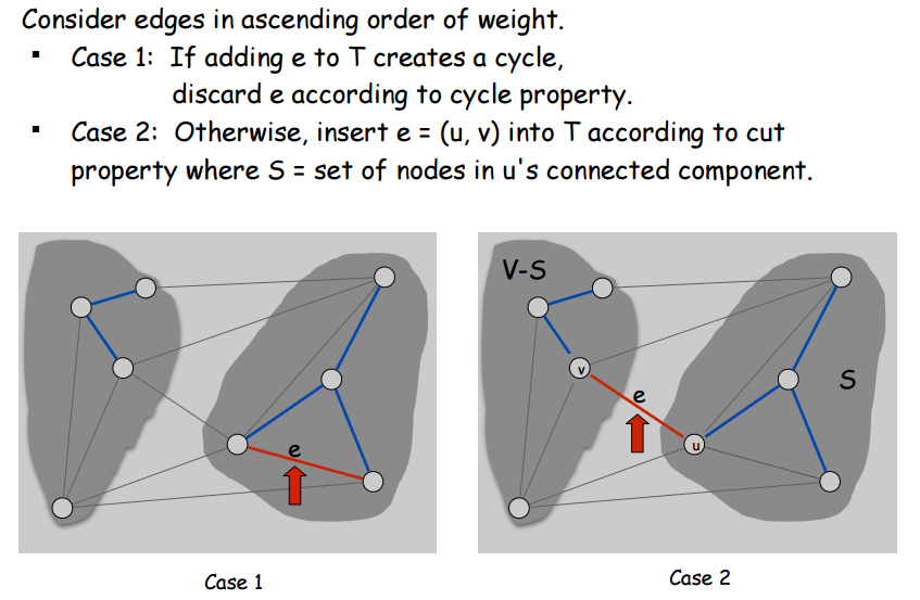
Just like Prim’s algorithm, the basic idea of Kruskal’s algorithm kind of just follows naturally from the properties of graphs that we talked about, the ones about the minimum values in cutsets (cut property) and maximum values in cycles (cycle property). Kruskal’s algorithm relies on the the property that the maximum value of any cycle can’t be in the MST. In short, you start by initializing the MST to empty. Then you sort all the edges in ascending order of cost. Then you literally just add edges that don’t create a cycle. That’s it. The tricky thing to design is just the part about always knowing whether an edge creates a cycle in your MST, which on the face of it, seems like something that should take a lot of time. That’s where the Union-Find data structure comes into play.
